Using a Stochastic Lambert Solver for GTOC1
Last time TR 2990 WX for scientific computing we showed how a 100 CPU Spark cluster may be replaced by a single CPU without any loss of performance for the Messenger-Full GTOP optimization problem. This time we will have a closer look at the GTOC1 problem GTOC1 and its approximation as part of the GTOP database. GTOC1 aims to remove a threat for planet earth caused by an asteroid headed in our direction. A small spaceship using an highly efficient low thrust ion engine is sent to hit the asteriod with so much force it will alter its course. “Force” means high impact speed at the asteroid at the “right” angle while maintaining as much mass as possible – which means use only a minimal amount of propellant. Planet gravity assist (GA) maneuvers help to achieve this goal. In the GTOP database there is simplified version of this problem GTOP - GTOC1 using a fixed planet flyby sequence approximating the low thrust engine fuel consumption by using the delta velocities (DVs) which need to to be applied at the flybys in addition to the DVs we get for free from the gravity of the planets. Since the given maximal thrust for GTOC1 is very low, this approximation works quite well. But if you compare the results from the competition (1.890.000 for the winning solution submitted by JPL) and the GTOP result 1581.950 GTOP - GTOC1 there is quite a gap. Why is this the case? We used techniques to fully utilize the AMD 2990WX CPU introduced in the last blog TR 2990 WX for scientific computing to answer this question.
Can the JPL Result for GTOC1 be Confirmed?
The real GTOC1 problem is much harder to solve compared to its GTOP counterpart for the following reasons:- The model (continuous thrust) is harder to compute, we need an integrator applied to the differential equations describing movement in space under continuous thrust.
- The planet sequence is not fixed.
- The time constraints don’t refer to single legs but to the whole mission.
In New GTOC1 Solution we see a solution by Team Jena slightly better than the JPL one, obtained by a search process which also determines the planet sequence, not only the timing of the transfers. We validated this solution which can be seen as an additional confirmation that 1.890.000 is a valid result. Since Lambert approximations were used during search, there is no explanation yet for the value gap to the best GTOP solution.
Can solutions of the real GTOC1 problem be validated by the GTOP GTOC1 problem?
To answer this question we slightly modified the GTOP code to support arbitrary (but fixed) planet sequences. We surprisingly found out that GTOP assigned high dv values to real GTOC1 solutions. Which means there must be an issue with the Lambert algorithm used. The GTOP GTOC1 code uses Lambert.cpp, but for the Jena GTOC1 solution we used the newer Lambert code lambert_problem.cpp . Main practical difference is that the newer code offers all possible solutions, the old code chooses the locally “best” solution. Problem is that in the context of flyby sequences the “best” Lambert solution is dependent on the neighbor legs. So the Lambert solutions chosen by the old algorithm are simply not the optimal ones for the whole sequence.
Selecting the Optimal Lambert Solutions for a Flyby Sequence
Using a search algorithm you may simply apply all Lambert solutions filtering the bad ones later while pruning branches having the lowest value assigned (Beam Search). Using direct optimization (as in the GTOP database) you have to find the optimal combination of solutions for the whole sequence as result of an “inner” optimization process. There may be millions of combinations for long sequences of multi revolution transfers, so we have to solve a complex sub problem while determining the DVs related to a set of specific transfer timings. But do we really have to do this?Replacing a Nested Optimization Problem by Using a Stochastic Target Function
Instead of solving the nested optimization problem which would be very slow we could modify the target function to generate random values based on a random selection from the solutions of the Lambert problems for each leg. Locally good Lambert solutions have to be selected with a much higher probability than the ones which are locally inferior. To estimate the “quality” of a specific Lambert solution we used the delta velocity subtracting outgoing from incoming spaceship velocity at the flybys neglecting the gravity assists. In practice we found probability values generating the best overall Lambert solution of a sequence after a few (< 10) tries. We modified the mga.cpp code to use this stochastic lambert solver based on lambert_problem.cpp . This only works if our optimization algorithm is “robust” related to noise. CMA-ES has this property, we found out that using a “noisy” target function does slow down the overall optimization, but that the slowdown is acceptable. Both the optimization results of the old deterministic and the stochastic approach generate solutions (transfer timings) which can be used for the continuous thrust model as initial guess for the final transfer timings, although these timings should be optimized in a final optimization step using the continuous thrust model. Higher approximated target values usually also mean a better final result value.
We investigated the following four planet sequences:
- GTOP: EVEVEJSA
- JENA: EVVEVVEESJA
- JPL: EVEEEJSJA
- GMV: EEVEEJSA
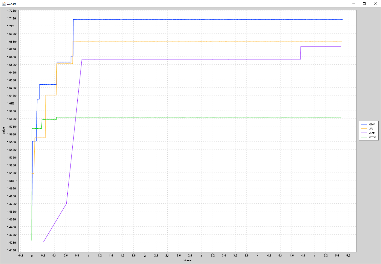
Here are the results using the original Lambert solver from the GTOP database
The Lambert solver used here is the original Lambert.cpp . All four experiments were performed simultaneously sharing a single CPU (AMD 2990wx) each executing 16 parallel threads. The original planet sequence marked GTOP - EVEVEJSA perfomed as expected reaching the best value 1.581.950 after about 25 minutes. EVEVEJSA turned out to be the worst sequence of the four tested, the GMV sequence being superior to the one from the JPL solution, and even better than the one from team Jena.
Here are the results using the stochastic Lambert solver:

The ranking is almost unchanged (beside now Jena > JPL), but the absolute values are largely increased, all “good” sequences now well above 1.800.000 . As before about 5 hours are needed until all four values are settled.
How to apply CMA-ES ?
Before we used the stochastic Lambert solver we optimized our usage of CMA-ES for the global optimization problem for a given planet sequence. Our final setting found the best solution of the original GTOP GTOC1 problem in less than 30 minutes using only 25% of our CPU.
As shown in our last blog TR 2990 WX for scientific computing the trick is generating many diverse initial guesses we feed as start values into the final optimization process. But this time instead of using a sub problem for the initial guesses we attacked the whole problem already at this stage.
In a parallel loop (16 threads) we generate preliminary CMA-ES solutions using random seeds and only 10000-30000 function evaluations depending on the length of the planet sequence.
Bad (< 1.450.000) preliminary solutions are filtered out.
Good preliminary solutions are used as seeds to a small number (about 3) of final CMA-ES runs using up to 2.000.000 evaluations.
The same algorithm was used in connection with the stochastic lambert solver. But we had to increase the filter limit (now < 1.600.000), since we got much better results.
Takeaways
To avoid expensive nested optimizations the inner optimization may be replaced by a stochastic function with carefully selected probabilities preferring good local solutions. Replacing the deterministic lambert solver used in GTOP – GTOC1 global optimization is only slightly slowed down but delivers superior results.The “gap” between GTOP-GTOC1 optimization results and “real” GTOC1 solutions can almost be closed and the optimization results provide a good basis for generating good continuous thrust solutions.
The old GTOP – GTOC1 benchmark is sufficient to evaluate the relative performance of different planet sequences, although specially for long sequences much more time is required to find good solutions using the deterministic lambert solver.
CMA-ES is sufficient for this problem, if you ensure diversity of initial guesses.
Appendix
The following limits were used for the optimizations:
- Dimension = 8 (GMV + GTOP)
- lower limit = [3000,14,14,14,14,100,366,300]
- upper limit = [10000,2000,2000,2000,2000,9000,9000,9000]
Dimension = 9 (JPL)
lower limit = [3000,14,14,14,14,100,366,300,300]
upper limit = [10000,2000,2000,2000,2000,6000,6000,6000,6000]
- Dimension = 11 (Jena)
- lower limit = [3000,14,14,14,14,14,14,100,366,300,300]
- upper limit = [10000,2000,2000,2000,2000,2000,2000,4000,4000,4000,4000]
GTOP - EVEVEJSA
- value = -1581950.212
- DVs = [3.4, 2.7, 0.0, 0.0, 0.0, 0.0, 0.0, 51.4]
- solution = [6810.42894, 168.3518, 1079.47355, 56.38753, 1044.0927, 3820.84585, 1044.32474, 3397.20717]
- time to find solution = 1584173.408409 ms
JENA - EVVEVVEESJA
- value = -1673184.703
- DVs = [2.8, 0.3, 0.2, 0.8, 0.0, 0.2, 0.0, 0.2, 0.6, 0.0, 50.9]
- solution = [9709.3523, 114.88036, 449.30007, 137.30591, 167.14522, 377.89481, 1043.8215, 3287.17736, 1100.59844, 3749.6718, 1875.19038]
- time to find solution = 1.7142722361067E7 ms
JPL - EVEEEJSJA
- value = -1680247.8
- DVs = [3.6, 1.7, 0.4, 0.0, 0.0, 0.0, 0.0, 0.0, 52.4]
- solution = [9681.00242, 149.32916, 668.38589, 1826.20633, 1826.20632, 500.55913, 486.05906, 4687.63598, 5212.84771]
- time to find solution = 2630874.751098 ms
GMV - EEVEEJSA
- value = -1708327.776
- DVs = [0.0, 0.6, 0.0, 0.5, 0.3, 0.0, 0.3, 51.2]
- solution = [3862.3599, 56.03464, 160.79779, 311.20351, 1095.7283, 6935.74335, 1206.49905, 2272.98044]
- time to find solution = 2660131.319524 ms
The Best Solutions Found Using the Stochastic Lambert Solver:
GTOP - EVEVEJSA
- value = -1775552.252
- DVs = [3.3, 0.1, 0.0, 0.0, 0.0, 0.0, 0.5, 51.9]
- solution = [7201.21904, 1583.71004, 367.13395, 1238.02714, 645.73245, 2343.03139, 996.59049, 3059.5073]
- time to find solution = 6581644.158691 ms
JENA - EVVEVVEESJA
- value = -1813613.878
- DVs = [2.8, 0.0, 0.0, 0.0, 0.0, 0.0, 0.0, 0.4, 0.0, 0.0, 51.0]
- solution = [7138.80635, 1555.67115, 947.97346, 1094.06006, 1087.87562, 1387.98293, 586.23478, 1562.64078, 996.52988, 3769.06163, 1888.30131]
- time to find solution = 8695902.942946 ms
JPL - EVEEEJSJA
- value = -1810572.908
- DVs = [2.8, 0.7, 0.0, 0.0, 0.4, 0.0, 0.0, 0.0, 52.6]
- solution = [7774.56731, 1593.25094, 1836.46182, 1578.8508, 1387.43318, 487.88568, 484.72706, 3287.27722, 539.04467, 2664.44376, 999.1674]
- time to find solution = 4561174.349158 ms
GMV - EEVEEJSA
- value = -1828322.685
- DVs = [2.5, 0.4, 0.0, 0.0, 0.0, 0.0, 0.0, 51.7]
- solution = [4847.96034, 883.2232, 1274.85615, 1796.9766, 1191.97604, 3300.43704, 956.56873, 3175.64633]
- time to find solution = 1.8461466498967E7 ms


Comments
Post a Comment