Ant Colony Optimization or CMA-ES, what is the Best Approach for Space Mission Design?
Open source real world optimization benchmarks hard enough to drive existing methods towards their limits are extremely rare. ESA’s Messenger full mission benchmark GTOP Task Messenger Full fulfills this criteria and therefore is currently a kind of reference problem to evaluate the effectiveness of optimization methods. It resembles an accurate model of Messengers full mission trajectory, so its solution is of real value for space mission planning. Currently the playing field is dominated by stochastic methods like ACO (Ant Colony Optimization), its commercial implementation Midaco (Mixed integer distributed ant colony optimization) and the open source CMA-ES (covariance matrix adaptation evolution strategy).
In MIDACO Messenger simple retry mechanisms for ACO/Midaco and CMA-ES are compared – resulting in a slight advantage for ACO/Midaco over CMA-ES. Simple retry mechanisms generally are not able to solve the Messenger Full problem. Based on ACO/Midaco a more sophisticated retry mechanism called MXHPC is presented, but no comparison to an equivalent method for CMA-ES is shown.
We provide this missing comparison using a retry method for CMA-ES which is as sophisticated as MXHPC for ACO/Midaco.
numactl -l -N0 ant TestRun | tee TestResult1.txt &
sleep 0.01
numactl -l -N2 ant TestRun | tee TestResult2.txt &
sleep 0.01
numactl -l ant TestRun | tee TestResult3.txt &
sleep 0.01
numactl -l ant TestRun | tee TestResult4.txt &
sleep 0.01
numactl -l -N0 ant TestRun | tee TestResult5.txt &
sleep 0.01
numactl -l -N2 ant TestRun | tee TestResult6.txt &
sleep 0.01
numactl -l ant TestRun | tee TestResult7.txt &
sleep 0.01
numactl -l ant TestRun | tee TestResult8.txt &
The 2990WX will perform 8 test runs in parallel – we configured each of the the runs to execute 8 CMA-ES executions in parallel each using 8 threads. Note that in this configuration CMA-ES doesn’t need to be parallelized itself although our CMA-ES implementation supports parallelization. The overhead is much reduced when executing single threaded CMA-ES runs in parallel. “tee” is used to split the output into separate files and to the terminal. “numactl” is used to assign 4 tasks to the two NUMA nodes having direct memory access. Experiments have shown this way the disadvantage having to use two NUMA nodes without direct memory access is minimized. The “sleep” calls are necessary to make sure each test run is started at a different time to make sure the pseudo random generator used is seeded differently each time.
Black box optimization is much easier to apply, but for hard problems it can be very resource demanding. Sometimes it is worth to split the original problem and solve a sub problem first. The white box approach referenced above uses a single CPU, the Midaco based black box solution needs a 100-CPU cluster. Nevertheless: An efficient black box solution would of course be preferable. It can directly be reused for other problems, no heuristics based adaption is required. Beside that: not all optimization problems have an exploitable internal structure. Therefore we will present such an efficient black box optimization method in the following section. After that we will again investigate a white box approach, one that substitutes discrete decision variables by converting the problem function into a heuristic based stochastic function. A black box mixed integer approach like Midaco learns the probability distribution for discrete decision variables by using “pheromones”, where we use domain specific information to simulate this probability distribution. A comparison with Midaco should be possible, as soon as a new version of the GTOP benchmark is released in 2019.
Crossover sets the initial value, limits the boundaries and determines the CMA-ES initial step size sigma parameter vector for the descendant.
The sigma value is similar to the Midaco Qstart parameter, but here it is individually set for each input variable. The boundaries and the sigma vector are derived from the difference of the two input vectors of the two ancestor solutions. This means input values already “settled” - similar in both ancestor input vectors - are more restricted as the other input variables.
The descendant CMA-ES run is initialized with one of the ancestor input vectors - we choose always the worse solution for initialization here. Crossover is applied after the initialization phase, but we continue to execute retries with a random initial input vector and initial boundaries to avoid getting caught by local minima. The rate crossover is performed in relation to random retries is a configuration parameter of GCMA-ES. Two GCMA-ES parameters determine how the boundaries / sigma values are derived from the difference vector of the two ancestor solutions. A stochastic mapping is used here to support diversification. Additional GCMA-ES parameters cover the crossover selection process.
To compare GCMA-ES with MXHPC using execution time is probably a bad idea since it is processor dependent. We used the AMD 2990WX to evaluate GCMA-ES, for MXHPC a 100 CPU Spark cluster was used. Instead of execution time we can use the number of function evaluations.
From the next diagram we see, that our CPU computed about 8 * 4 * 10⁹ evaluations in the 5 hour test period, 4 * 10⁹ evaluations for each test run executed in parallel. Only two minima (with minor variations) are reached, one at about 2.4, one at the absolute minimum of 1.958.

For MXHPC ten test runs were documented, all but one used more than 60 * 10⁹ evaluations. Best result was 2.025. We will check how many results lower than a certain threshold GCMA-ES can compute using the same 60 * 10⁹ evaluations.
We restart GCMA-ES if we either find a value better than the threshold, or an evaluation limit is reached. We compute the probability distribution of the number of solutions below the threshold for different threshold and evaluation limit values.
Here is the distribution for threshold = 2.0 and evaluation limits 1*10⁹, 2*10⁹ and 3*10⁹ . This threshold is below the best result achieved by MXHPC. GCMA-ES is able to find on average more than 20 solutions < 2.0 using 60 * 10⁹ evaluations.

Finally lets lower the threshold to 1.9585, a value below the one listed as optimum at the GTOP page. That such a solution exists was first reported by Mincheng Zuo (China Uni. of Geoscience), see Best Messenger Full Solution .
Even using this “below the old record” threshold, GCMA-ES finds on average about 12 solutions < 1.9585 using 60 * 10⁹ evaluations.

These results give a clear indication which algorithm is superior in solving the GTOP messenger full benchmark problem.
In the picture below we see the spaceship (red) approaching the asteroid (orange) coming from Jupiter using a retrograde orbit to maximize its impact.

A video of the whole mission can be seen here GTOP GTOC1 video .
Is the reason for this “result gap” the impulse / Lambert approximation? We can close the gap by modifying GTOP-GTOC1 so that it is better suited to solve GTOC1:
The original GTOC1 problem doesn’t fix the sequence of planets visited, the sequence used for GTOP-GTOC1 is not optimal. Team Jena found better sequence New GTOC1 Solution We adapted GTOP-GTOC1 to use the Team Jena planet sequence EVVEVVEESJA.
GTOP-GTOC1 uses a simplified version of the Lambert algorithm which delivers only the locally best Lambert solution. There is a new version of the Lambert algorithm lambert_problem.cpp delivering all solutions instead. Locally optimal Lambert solutions are not guaranteed to be optimal in the context of a Lambert sequence connected by gravity assist maneuvers. We adapted GTOP-GTOC1 to use this new Lambert algorithm using maximal number of revolutions = 5.
Limits should be adjusted so that the overall time limit doesn’t increase compared to GTOP-GTOC1, we choose:
lower limit = [3000,14,14,14,14,14,14,100,366,300,300]
upper limit = [10000,2000,2000,2000,2000,2000,2000,4000,4000,4000,4000]
Deciding which Lambert solution to use for each trajectory leg introduces additional discrete integer decision variables to the solution vector. This transforms the problem into a mixed integer optimization problem.
As limits for the integer decision variables we could use
lower limit = [0,0,0,0,0,0,0,0,0,0] and
upper limit (inclusive) = [10,10,10,10,10,10,10,0,0,0]
as for the outer planet transfers the Lambert solver in practice only offers one solution. The number of transfers is dependent on the time of flight.
MXHPC supports discrete integer decision variables without relaxation, but GCMA-ES does not. We could relax the discrete variables to real values and use rounding to convert these back to integers when we have to select a Lambert solution. This would introduce discontinuities to the function to be optimized.
CMA-ES is a stochastic algorithm capable of handling discontinuities. But we wouldn’t utilize the fact that the different Lambert solutions are associated to different local delta velocity (DV) values. Although choosing always the Lambert solution with the lowest local DV value – as done by the old GTOP GTOC1 benchmark - is not guaranteed to deliver a globally optimal solution, this value is a strong indication about the probability a Lambert solution is part of such a global optimum. Low local DV value means: There is a high probability this Lambert solution is part of the global optimum.
So instead of converting the problem into a mixed integer one, we keep the original continuous input vector and convert the function to be optimized into a stochastic one. CMA-ES is able to optimize “noisy” functions, so this shouldn’t be a problem. Each time we have to choose a Lambert solution, we randomly chose one, but strongly prefer Lambert solutions with a low local DV value.
This approach has two advantages:
Here we have the J score reached after x hours:

The next diagram shows the J score reached after n function evaluations:

We will check how many results higher than a certain J-threshold GCMA-ES can compute using the 60 * 10⁹ evaluations (the same number used for Messenger-Full). We restart GCMA-ES if we either find a value better than the threshold, or an evaluation limit is reached. We compute the probability distribution of the number of solutions below the threshold for different threshold and evaluation limit values.
Here is the distribution for threshold J = 1850000 and evaluation limits 3*10⁹, 4*10⁹ and 5*10⁹ , the winning score in the original competition GTOC1 Results .

Here is the distribution for threshold J = 1.880.000 and evaluation limits 3*10⁹, 4*10⁹ and 5*10⁹. No team in the original competition reached this score. But note that the best trajectories found violate the 30 years mission time limit from the original competition and instead of low/continuous thrust we use impulses here.

We find 2 results with J > 1.880.000 using 60*10^9 evaluations on average.
[7071.70229865, 1624.94936996, 898.77131464, 845.77519091, 1149.79247469, 1181.9935484, 678.99624647, 2288.17876494, 957.92741851, 3708.97332311, 3133.46677205]
with DV values:
DV0 = 2.503413740690902 – 2.5 = 0.00341
DV1 = 2.706695383380975E-6
DV2 = 4.835477129816468E-6
DV3 = 1.192128262772485E-7
DV4 = 4.3576198844874625E-6
DV5 = 1.0350682781989917E-6
DV6 = 2.5130877965295895E-6
DV7 = 1.5422751786786648E-6
DV8 = 9.455994920415378E-7
DV9 = 0.0016189542152744707
Target impact velocity = 51.773729882711045
Sum of the DVs = 0.005050749942145938
J = 1893779.7225388156
Number of solutions delivered from the new Lambert Solver:
[11, 11, 5, 9, 11, 5, 11, 1, 1, 1]
Index of the chosen Lambert solution:
[9, 3, 3, 8, 6, 0, 2, 0, 0, 0]
J = 1893779 is better than the result achieved by the winning team JPL, J = 1850000. Because of the very low DV values, conversion into a low thrust / continuous thrust trajectory should be easy. But this solution doesn’t fulfill the original mission time constraint of 30 years of the original GTOC1 competition.
The first diagram shows the result value reached for 16 GCMA-ES runs using about 2x11 hours, 8 runs executed on parallel on the TR 2990WX processor.

Observations:

Probably the solution landscape is “smoothed” a bit using the new Lambert solver which speeds up the convergence. This should be further investigated.
Finally we will check how many results better than a certain threshold value GCMA-ES can compute using 60 * 10⁹ evaluations. We restart GCMA-ES if we either find a value better than the threshold, or an evaluation limit is reached. We compute the probability distribution of the number of solutions below the threshold for different threshold and evaluation limit values.
Here is the distribution for threshold value = 1.93 and evaluation limits 1*10⁹, 2*10⁹ and 3*10⁹
 About 13 results better than 1.93 are to be expected using 60 * 10⁹ evaluations.
Best Solution found:
Solution = [2036.88535842, 4.05, 0.54363562, 0.64096897, 450.83254143, 224.69412634, 222.8513383, 266.07218374, 357.80562972, 534.53186968, 0.30354342, 0.69317052, 0.69193936, 0.73764561, 0.82876394, 0.1123704, 1.58401789, 1.1, 1.05, 1.05, 1.05, 2.75802556, 1.57072851, 2.08319586, 1.59521739, 1.58135447]
Function Value = 1.92492
DV values:
DV: 0 = 4.05
DV: 1 = 0.154967
DV: 2 = 8.05468e-05
DV: 3 = 0.425502
DV: 4 = 0.077342
DV: 5 = 0.205197
DV: 6 = 0.190106
DV: 7 = 0.871724
In MIDACO Messenger simple retry mechanisms for ACO/Midaco and CMA-ES are compared – resulting in a slight advantage for ACO/Midaco over CMA-ES. Simple retry mechanisms generally are not able to solve the Messenger Full problem. Based on ACO/Midaco a more sophisticated retry mechanism called MXHPC is presented, but no comparison to an equivalent method for CMA-ES is shown.
We provide this missing comparison using a retry method for CMA-ES which is as sophisticated as MXHPC for ACO/Midaco.
- Note 1: Our CMA-ES implementation - used with a simple retry mechanism - produces similar results to the one listed in MIDACO Messenger . Therefore our sophisticated CMA-ES retry method should perform in a similar manner when used with any open source CMA-ES implementation.
- Note 2: CMA-ES cannot be applied directly to mixed integer problems without relaxation of the discrete integer variables to continuous values. Further below we will have a closer look at a specific mixed integer space mission design problem. We will show how CMA-ES can still be used here using a whitebox approach. Instead of applying continuous + integer decision variables to a deterministic function we apply only the continuous variables to a stochastic (noisy) function representing the same problem.
How to fully utilize the 32 Cores of the 2990WX
Our implementation uses Java calling C++ via JNI. We export our Eclipse run configuration as ant build.xml file called via the following shell script:numactl -l -N0 ant TestRun | tee TestResult1.txt &
sleep 0.01
numactl -l -N2 ant TestRun | tee TestResult2.txt &
sleep 0.01
numactl -l ant TestRun | tee TestResult3.txt &
sleep 0.01
numactl -l ant TestRun | tee TestResult4.txt &
sleep 0.01
numactl -l -N0 ant TestRun | tee TestResult5.txt &
sleep 0.01
numactl -l -N2 ant TestRun | tee TestResult6.txt &
sleep 0.01
numactl -l ant TestRun | tee TestResult7.txt &
sleep 0.01
numactl -l ant TestRun | tee TestResult8.txt &
The 2990WX will perform 8 test runs in parallel – we configured each of the the runs to execute 8 CMA-ES executions in parallel each using 8 threads. Note that in this configuration CMA-ES doesn’t need to be parallelized itself although our CMA-ES implementation supports parallelization. The overhead is much reduced when executing single threaded CMA-ES runs in parallel. “tee” is used to split the output into separate files and to the terminal. “numactl” is used to assign 4 tasks to the two NUMA nodes having direct memory access. Experiments have shown this way the disadvantage having to use two NUMA nodes without direct memory access is minimized. The “sleep” calls are necessary to make sure each test run is started at a different time to make sure the pseudo random generator used is seeded differently each time.
Black Box / White Box Optimization
Black box optimization takes an optimization problem as it is, where white box optimization exploits its internal structure. For GTOP Task Messenger Full a state of the art black box approach is described in MIDACO Messenger , a white box approach can be found here Messenger Full White Box .Black box optimization is much easier to apply, but for hard problems it can be very resource demanding. Sometimes it is worth to split the original problem and solve a sub problem first. The white box approach referenced above uses a single CPU, the Midaco based black box solution needs a 100-CPU cluster. Nevertheless: An efficient black box solution would of course be preferable. It can directly be reused for other problems, no heuristics based adaption is required. Beside that: not all optimization problems have an exploitable internal structure. Therefore we will present such an efficient black box optimization method in the following section. After that we will again investigate a white box approach, one that substitutes discrete decision variables by converting the problem function into a heuristic based stochastic function. A black box mixed integer approach like Midaco learns the probability distribution for discrete decision variables by using “pheromones”, where we use domain specific information to simulate this probability distribution. A comparison with Midaco should be possible, as soon as a new version of the GTOP benchmark is released in 2019.
Sophisticated Retry of Stochastic Optimization Methods:
A simple retry method works as follows:
We set a threshold target value and a function evaluation limit and then execute the optimization algorithm in a loop. The execution is stopped if either the threshold value or the evaluation limit is reached, then we restart the execution to try again.A sophisticated retry method may add the following techniques:
- Store a history of past
- Use this history to “exchange” information from previous runs to configure the next run.
- Use this history to dynamically stop the execution before the evaluation limit is reached if the value reached so far is bad compared to the values reached at this point in previous runs. A a similar idea applied for tree search is called “beam search”.
- Incrementally increase the final evaluation limit over time to produce the first history entries fast. Quality of history entries will improve over time as the evaluation limit increases, but the information from early entries is already valuable for (1) and (2). A similar idea applied in other areas is called “iterative deepening”.
GCMA-ES
The retry method for CMA-ES used in our comparison is called GCMA-ES (genetic CMA-ES), because we can view the history of past retries as population in a genetic algorithm. We only use two genetic operators, selection and crossover. Mutation may be useful in this context too, but it is not included in GCMA-ES yet.Selection
Only a limited number of highly ranked retries survive each generation. Before a retry is added to the population we check for similarity with existing members using the euclidean distance of the two solutions normalized to the interval [0,1] using the boundaries. If both of the two function values and the euclidian distance of the normalized solutions is below a threshold, only the better solution of the two will survive in the population. This avoids accumulating equivalent solutions which would reduce diversification. The distance threshold and the population size are configuration parameters of GCMA-ES.Initialization
At the beginning each CMA-ES retry is seeded with a random initial input vector and uses the original boundaries of the problem. Each CMA-ES run performs a limited number of function applications and delivers a solution which maps an input vector to the best value found in this run. We use the same CMA-ES initial step size sigma parameter for all variables of the input vector, which is a configuration parameter of GCMA-ES. The CMA-ES sigma parameter has some similarity to the Midaco Qstart parameter.Crossover
Two ancestor solutions are selected for crossover where higher ranked solutions have a higher probability to be selected.Crossover sets the initial value, limits the boundaries and determines the CMA-ES initial step size sigma parameter vector for the descendant.
The sigma value is similar to the Midaco Qstart parameter, but here it is individually set for each input variable. The boundaries and the sigma vector are derived from the difference of the two input vectors of the two ancestor solutions. This means input values already “settled” - similar in both ancestor input vectors - are more restricted as the other input variables.
The descendant CMA-ES run is initialized with one of the ancestor input vectors - we choose always the worse solution for initialization here. Crossover is applied after the initialization phase, but we continue to execute retries with a random initial input vector and initial boundaries to avoid getting caught by local minima. The rate crossover is performed in relation to random retries is a configuration parameter of GCMA-ES. Two GCMA-ES parameters determine how the boundaries / sigma values are derived from the difference vector of the two ancestor solutions. A stochastic mapping is used here to support diversification. Additional GCMA-ES parameters cover the crossover selection process.
Comparison of GCMA-ES with MXHPC
For GCMA-ES we performed 32 = 4 * 8 runs for about 5 hours, where 8 of them were executed in parallel on a single CPU AMD TR 2990WX. The experiment took about 20 (= 4 * 5) hours.To compare GCMA-ES with MXHPC using execution time is probably a bad idea since it is processor dependent. We used the AMD 2990WX to evaluate GCMA-ES, for MXHPC a 100 CPU Spark cluster was used. Instead of execution time we can use the number of function evaluations.

From the next diagram we see, that our CPU computed about 8 * 4 * 10⁹ evaluations in the 5 hour test period, 4 * 10⁹ evaluations for each test run executed in parallel. Only two minima (with minor variations) are reached, one at about 2.4, one at the absolute minimum of 1.958.

For MXHPC ten test runs were documented, all but one used more than 60 * 10⁹ evaluations. Best result was 2.025. We will check how many results lower than a certain threshold GCMA-ES can compute using the same 60 * 10⁹ evaluations.
We restart GCMA-ES if we either find a value better than the threshold, or an evaluation limit is reached. We compute the probability distribution of the number of solutions below the threshold for different threshold and evaluation limit values.
Here is the distribution for threshold = 2.0 and evaluation limits 1*10⁹, 2*10⁹ and 3*10⁹ . This threshold is below the best result achieved by MXHPC. GCMA-ES is able to find on average more than 20 solutions < 2.0 using 60 * 10⁹ evaluations.

Finally lets lower the threshold to 1.9585, a value below the one listed as optimum at the GTOP page. That such a solution exists was first reported by Mincheng Zuo (China Uni. of Geoscience), see Best Messenger Full Solution .
Even using this “below the old record” threshold, GCMA-ES finds on average about 12 solutions < 1.9585 using 60 * 10⁹ evaluations.

These results give a clear indication which algorithm is superior in solving the GTOP messenger full benchmark problem.
Disadvantages / Advantages of GCMA-ES compared to MXHPC
To summarize the results we first list here the disadvantages of GCMA-ES:
- All test runs converge to a value < 2.42 which is significantly worse compared to the worst result from the 10 test run results listed for MXHPC.
- There are many global parameters for GCMA-ES where it is not verified yet that the parameters optimal for Messenger Full are useful also for other problems. Other hard optimization problems should be tried to find more general parameters for GCMA-ES.
- Neither a public open source implementation nor a commercial product is available yet.
Advantages of GCMA-ES are:
- No final optimization needed, there is a high chance to find the global minimum. All 10 test runs reported for MXHPC failed (marginally) here.
- Using the same amount of function evaluations – 60 * 10⁹ – GCMA-ES computes on average about 24 solutions each better than the best solution found in the 10 MXHPC test runs.
- Instead of using a 100 CPU Sparc cluster a single desktop processor (the AMD TR 2990WX) can perform 8 test runs in parallel in 5 hours. “numactl” should be used to configure the 4 NUMA nodes of the processor in an optimal way. Using a single process on a single CPU simplifies the information exchange between multiple CMA-ES retries. In our tests after 5 hours we found each time the optimal solution 1.958 in at least one of the 8 results.
Solving a Mixed Integer Space Mission Design Optimization Problem
Not all optimization problems are restricted to continuous input variables, sometimes discrete decisions have to be performed. Thesis_Schlueter provides a nice introduction into this issue. Here we will introduce such a problem and solve it using GCMA-ES. CMA-ES (as ACO) is a stochastic optimization algorithm suitable to be applied to hard optimization problems. Sophisticated retry mechanisms like MXHPC for ACO and GCMA-ES for CMA-ES further enhance the capabilities of the algorithms they are based on. MXHPC can directly solve problems including discrete integer variables. Since GCMA-ES doesn’t have this capability we have to use a “white box” solution here.GTOP-GTOC1 Revisited
The open source space mission design optimization benchmark GTOP - GTOC1 is the basis of our investigation. GTOC1 was the first of a series of competitions where the best space mission design teams of the world compete almost each year. Task is to compute a flyby sequence using gravity assists at the planets to hit a target asteroid posing a threat to earth with as much “force” as possible to protect our planet. In the original task a low thrust engine is used, but its maximal thrust limit is low enough such that the sequence can be approximated with high accuracy using high thrust impulses. Easy to compute Lambert transfers – corresponding to Keplerian orbits – are used to approximate the trajectory legs. The space design optimization benchmark GTOP - GTOC1 uses this Lambert approximation – but the best result found so far is significantly lower than the best “real” GTOC1 solution from JPL GTOC1 Results .In the picture below we see the spaceship (red) approaching the asteroid (orange) coming from Jupiter using a retrograde orbit to maximize its impact.

A video of the whole mission can be seen here GTOP GTOC1 video .
Is the reason for this “result gap” the impulse / Lambert approximation? We can close the gap by modifying GTOP-GTOC1 so that it is better suited to solve GTOC1:
The original GTOC1 problem doesn’t fix the sequence of planets visited, the sequence used for GTOP-GTOC1 is not optimal. Team Jena found better sequence New GTOC1 Solution We adapted GTOP-GTOC1 to use the Team Jena planet sequence EVVEVVEESJA.
GTOP-GTOC1 uses a simplified version of the Lambert algorithm which delivers only the locally best Lambert solution. There is a new version of the Lambert algorithm lambert_problem.cpp delivering all solutions instead. Locally optimal Lambert solutions are not guaranteed to be optimal in the context of a Lambert sequence connected by gravity assist maneuvers. We adapted GTOP-GTOC1 to use this new Lambert algorithm using maximal number of revolutions = 5.
Limits should be adjusted so that the overall time limit doesn’t increase compared to GTOP-GTOC1, we choose:
lower limit = [3000,14,14,14,14,14,14,100,366,300,300]
upper limit = [10000,2000,2000,2000,2000,2000,2000,4000,4000,4000,4000]
Deciding which Lambert solution to use for each trajectory leg introduces additional discrete integer decision variables to the solution vector. This transforms the problem into a mixed integer optimization problem.
As limits for the integer decision variables we could use
lower limit = [0,0,0,0,0,0,0,0,0,0] and
upper limit (inclusive) = [10,10,10,10,10,10,10,0,0,0]
as for the outer planet transfers the Lambert solver in practice only offers one solution. The number of transfers is dependent on the time of flight.
MXHPC supports discrete integer decision variables without relaxation, but GCMA-ES does not. We could relax the discrete variables to real values and use rounding to convert these back to integers when we have to select a Lambert solution. This would introduce discontinuities to the function to be optimized.
CMA-ES is a stochastic algorithm capable of handling discontinuities. But we wouldn’t utilize the fact that the different Lambert solutions are associated to different local delta velocity (DV) values. Although choosing always the Lambert solution with the lowest local DV value – as done by the old GTOP GTOC1 benchmark - is not guaranteed to deliver a globally optimal solution, this value is a strong indication about the probability a Lambert solution is part of such a global optimum. Low local DV value means: There is a high probability this Lambert solution is part of the global optimum.
So instead of converting the problem into a mixed integer one, we keep the original continuous input vector and convert the function to be optimized into a stochastic one. CMA-ES is able to optimize “noisy” functions, so this shouldn’t be a problem. Each time we have to choose a Lambert solution, we randomly chose one, but strongly prefer Lambert solutions with a low local DV value.
This approach has two advantages:
- We no longer loose the information the local DV value provides for the optimization process.
- We keep the continuous input vector and can apply CMA-ES without relaxation.
- We cannot view the function as “black box”, instead we have to apply a heuristic to convert it into a stochastic function using the local DV value associated to the Lambert transfers.
Results
Using the GCMA-ES algorithm we performed 16 = 2 * 8 runs for about 12 hours, where 8 of them were executed in parallel on a single CPU AMD TR 2990WX. The experiment took about 1 day (2 * 12 hours).Here we have the J score reached after x hours:

The next diagram shows the J score reached after n function evaluations:

We will check how many results higher than a certain J-threshold GCMA-ES can compute using the 60 * 10⁹ evaluations (the same number used for Messenger-Full). We restart GCMA-ES if we either find a value better than the threshold, or an evaluation limit is reached. We compute the probability distribution of the number of solutions below the threshold for different threshold and evaluation limit values.
Here is the distribution for threshold J = 1850000 and evaluation limits 3*10⁹, 4*10⁹ and 5*10⁹ , the winning score in the original competition GTOC1 Results .

Here is the distribution for threshold J = 1.880.000 and evaluation limits 3*10⁹, 4*10⁹ and 5*10⁹. No team in the original competition reached this score. But note that the best trajectories found violate the 30 years mission time limit from the original competition and instead of low/continuous thrust we use impulses here.

We find 2 results with J > 1.880.000 using 60*10^9 evaluations on average.
Best GTOC1 result found
GCMA-ES delivered a solution:[7071.70229865, 1624.94936996, 898.77131464, 845.77519091, 1149.79247469, 1181.9935484, 678.99624647, 2288.17876494, 957.92741851, 3708.97332311, 3133.46677205]
with DV values:
DV0 = 2.503413740690902 – 2.5 = 0.00341
DV1 = 2.706695383380975E-6
DV2 = 4.835477129816468E-6
DV3 = 1.192128262772485E-7
DV4 = 4.3576198844874625E-6
DV5 = 1.0350682781989917E-6
DV6 = 2.5130877965295895E-6
DV7 = 1.5422751786786648E-6
DV8 = 9.455994920415378E-7
DV9 = 0.0016189542152744707
Target impact velocity = 51.773729882711045
Sum of the DVs = 0.005050749942145938
J = 1893779.7225388156
Number of solutions delivered from the new Lambert Solver:
[11, 11, 5, 9, 11, 5, 11, 1, 1, 1]
Index of the chosen Lambert solution:
[9, 3, 3, 8, 6, 0, 2, 0, 0, 0]
J = 1893779 is better than the result achieved by the winning team JPL, J = 1850000. Because of the very low DV values, conversion into a low thrust / continuous thrust trajectory should be easy. But this solution doesn’t fulfill the original mission time constraint of 30 years of the original GTOC1 competition.
Messenger Full with new Lambert Solver
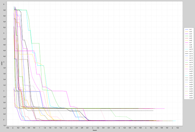
Finally lets have a look what happens if we apply the new Lambert solver to the messenger full problem:The first diagram shows the result value reached for 16 GCMA-ES runs using about 2x11 hours, 8 runs executed on parallel on the TR 2990WX processor.

Observations:
- 15 out of the 16 runs converge very fast to a value below the old optimum 1.958
- The best value 1.925 is not much better than the result reached using the old lambert solver.
- Execution time is higher than using the old Lambert solver, may be because we used an unnecessary high maximal number of revolutions = 5.

Probably the solution landscape is “smoothed” a bit using the new Lambert solver which speeds up the convergence. This should be further investigated.
Finally we will check how many results better than a certain threshold value GCMA-ES can compute using 60 * 10⁹ evaluations. We restart GCMA-ES if we either find a value better than the threshold, or an evaluation limit is reached. We compute the probability distribution of the number of solutions below the threshold for different threshold and evaluation limit values.
Here is the distribution for threshold value = 1.93 and evaluation limits 1*10⁹, 2*10⁹ and 3*10⁹

Best Solution found:
Solution = [2036.88535842, 4.05, 0.54363562, 0.64096897, 450.83254143, 224.69412634, 222.8513383, 266.07218374, 357.80562972, 534.53186968, 0.30354342, 0.69317052, 0.69193936, 0.73764561, 0.82876394, 0.1123704, 1.58401789, 1.1, 1.05, 1.05, 1.05, 2.75802556, 1.57072851, 2.08319586, 1.59521739, 1.58135447]
Function Value = 1.92492
DV values:
DV: 0 = 4.05
DV: 1 = 0.154967
DV: 2 = 8.05468e-05
DV: 3 = 0.425502
DV: 4 = 0.077342
DV: 5 = 0.205197
DV: 6 = 0.190106
DV: 7 = 0.871724
Takeways
- If you perform scientific experiments (simulation / search / optimization) and you use a processor like the AMD TR 2990 WX having NUMA nodes without direct memory access: Use "numactl -l -Nx" to assign tasks to the numa nodes with direct memory access until they are fully utilized.
- One TR AMD 2990 WX CPU is sufficient to solve the GTOP messenger full optimization benchmark using a new black box optimization algorithm called GCMA-ES. Previously a 100 CPU Spark cluster was required.
- Using a GCMA-ES based white box approach replacing integer decision variables by an heuristic stochastic problem function a modified GTOP GTOC1 problem can solved. This solution is very good compared to previous solutions of the GTOC1 task.
- The same GCMA-ES based white box approach simplifies the messenger full problem so that it is much easier to solve. GCMA-ES converges must faster. Why this is the case is subject of future research.


Comments
Post a Comment